NLP - Unsupervised Pretraining Models
Contents
1. Self-Supervised Pre-Training Models
The self-attention in transformers has been gaining popularity across the DL domain due to its high performance and versatility. Models that adopt the structure include BERT, GPT, ALBERT, ELECTra in the domain of NLP.
a. GPT-1

- Introduced special tokens for start of the sentence, end of the sentence, or deliminators to cater to diverse tasks of transfer learning
- No need to use task-specific models for each task
- Train the transformer with LM (Language Model), and use the pretrained transformer like a lego block to structure the model for a specific task
- Attach a vector for extraction, feed into the network, and use the altered extraction vector to yield the result

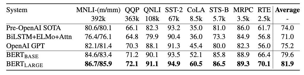
- Outperformed all other contemporary SOTA models in almost all tasks.
b. BERT

- GPT has the problem of not taking into account the sequences that come either before or after the current time period
- To solve this problem, BERT introduced MLM (Masked Language Model) for pretraining, a bi-directional language model. Usually in bi-directional models, the model can cheat by looking at the answers from future sequences. However, MLM prevents this by replacing a word with a [Mask] token. In speicifc, the researchers set the masking ratio to 15%, and within that 15% percent of masked words, left the masked token unchage 80% of the times, 10% of the times replaced the word with a random word, and for the other 10% kept the same sentence. This was because the model would not find a [Mask] token in the pretraining stage, and the researchers wanted the model to be prepared for such an environment
- Another type of dataset the reseachers used for pretraining was NSP (Next sentence Predition), in which task that the model has to decide whether the two sentence were together originally, or a stack of two random sentences.
- Used WordPiece embeddings
- For positional embedding, BERT did not use predifined sinusoidal functions. Rather, it uses trainable positional embedding
- When the model has two sequences to process, the model adds addtional embedding vector to the sequences. Add 0 to the first sequence for all embedding vectors, and 1 to the next sequence.
c. Pre-training and Fine Tuning of BERT

- Pretrain on MLM and NSP simultaneously. Use the [CLS] token to get the answer for NSP task, and the other outputs for MLM task.

- The process is similar for task-specific transfer learning, with changes on the format of input vector and the vectors the model uses to pin down the answer.
d. GPT-1 vs BERT
- Data Size for Pretraining
- GPT: BookCorpus (800M Words)
- BERT BookCorpus + Wikipedia (2500M Words)
- BERT learns A/B embedding (sentence differentiation) during pretraining
- Batch Size: Larger the better for performance
- GPT: 32000 words
- BERT: 128000 words
- BERT uses different learning rates for each fine-tuning experiments. GPT uses the same learning rate for all tasks
e. Machine Reading Comprehension for BERT
- BERT is not confined to predicting missing words. The model can be trained to understand a given passage and answer a question regarding that passage.
- Use [CLS] token to check if the answer is in the passge. Then the model specifies a start vector and an end vector, which were previously input vectors of a sequence. The phrase between the two vectors is the answer.
2. Advanced Self-Supervised Pre-Training Models
a. GPT-2
- Much larger than GPT-1, but still trained with LM
- High quality dataset
- Divided the weights of residual layer with
- Aimed for performing specific tasks on a zero-shot setting. The model does not need additional modification nor transfer learning to perform specific tasks.
- To summarize, ask the model “what is the summary of a given passage”
- To classify the sentiment, ask the model “what is the sentiment of a given sentence”
- We do not ask actual questions to the model. We rather add a token or a phrase such as TL;DL (too long did not read) to summarize, but the point is that any task is essentially presented in the form of a question, so we do not need different structures for different tasks.
b. ALBERT
The size of language models were getting gigantic, need to reduce the size while retaining decent performance. ALBERT suceeded in surpassing the SOTA models with a lighter model

Image Source
- Factorized Embedding Parameterization
reference
: Vocab size
: Hidden state dimension
: Word embedding dimension
- Hidden-state dimension should be the same as word embedding dimension due to the residual connection
- In order to transform the word embedding to
. However, if we factorize this into two vectors with the size of
and
, we can save up memory as long as
- Cross-layer Parameter Sharing
Many layers, can share parameters across layers

- Shared-FFN: sharing only the feed-forward parameters. Networks that process the
- Shared-attention: sharing only the attention parameters. Networks that produces the
- All-shared: sharing all
c. ELECTRA

- Similar to the idea of GAN
- Pretrain the encoder model as a discriminator, the main network
- The discriminator tries to find out if the generator, usually a small MLM model, replaced the word or not.

- Surpasses MLM models
d. Light-weight Models
Aims to use language models on light devices such as mobile devices.
- DistillBERT: learns on soft labels that the teacher model produced
- TinyBERT: tries to mimic the outputs within the learning stages such as the key vector transformation matrix. The dimension is different because TinyBERT is a smaller model. Uses fully connected layer to channel the output of the teacher model into the student model. The parameters of the fully connected layer is also trainable.